Chapter 5:              Calcium Carbonate Clusters

 

 

5.1    Introduction

 

“In eighteenth-century Newtonian mechanics, the three-body problem was insoluble. With the birth of general relativity around 1910 and quantum electrodynamics in 1930, the two-and three-body problems became insoluble. And within modern quantum field theory, the problem of zero bodies (vacuum) is insoluble. So, if we are out after exact solutions, no bodies at all is already too many.” – Prof. G. E. Brown, quoted in Computer Simulation in Material Science, 1996, p.77.

Calcite is the most abundant mineral found, comprising approximately 4% by weight of the Earth’s crust and is formed in many different geological environments.  The crystals of calcite can have thousands of different crystal forms by building on the hundreds of different basic shapes, like the positive rhombohedron, negative rhombohedron, steeply, moderately and slightly inclined rhombohedrons, various scalahedrons, prism and pinacoid.

The most common polymorphs of calcium carbonate are aragonite and calcite.  That is, they contain the same elements but they differ in crystal structure.  Aragonite is an orthorhombic structure, similar to a rectangle, except that the angles at the two opposing corners are about 75 degrees and 105 degrees.  Calcite has a trigonal structure.  Calcite and Aragonite are polymorphous to each other.    Sometimes, the crystals of Calcite and Aragonite are too small to be detected by the eye, and it is only possible to distinguish these two minerals by optical magnification.  The polymorphs are simply labeled as "Calcium Carbonate". The polymorph vaterite, which has a hexagonal structure, is extremely rare.  The mechanism responsible for the formation of the various polymorphs of calcium carbonate (CaCO₃); calcite, aragonite and vaterite, is still the subject of much research.

Calcite, the polymorph of CaCO₃, is used in a wide range of applications, like the construction industry (in the interiors of cathedrals, temples, and public buildings), in the manufacturing of fertilizers, and in the metal, glass, rubber and paint industries.  It is also used in some optical devices, like the Nicol prisms, which is used in polarizing microscopes.   Fig. 5.1 shows an image of dolomite and calcite crystallites taken through a polarizing microscope [61].    The color photograph is from the dinosaur bone collection and shows the fossilized teeth in a dinosaur.  Over time the spaces between the bones in the mouth begin to mineralize, forming calcite crystallites, dolomite, and other minerals.

The specific gravity of calcite is approximately 2.71 and the molecular weight is 100.09 amu.     The work in the past has been focused on determining physical properties of calcite by developing an empirical model that is based on the properties of bulk material.  A. Pavese et al. [18] used computational methods based on the quasi-harmonic approximation to calculate the temperature dependence of elastic constants and structural features of the crystal.  A. Skimmer [62] and R. K. Singh et al. [63] investigated the lattice dynamics of several types of molecular crystals, including CaCO₃.  Their approach was to use the Rigid Ion Model (RIM) as the interaction potential [18,64].

            There has also been interest in the mechanisms responsible for the growth of the observed crystalline structure.  A few researchers have begun using ab-initio calculations in the study of small clusters of calcite.  Y. Mao et al. [65] modeled the properties of the monomer and dimer of CaCO₃ by using ab-initio Hartee-Fock calculations.  The structures they achieved for the monomer and dimer agreed with the structures I found.  M. Catti et al. [66] determined the static crystal energy of calcite and its structure as functions of pressure by using all-electron periodic HF calculations for the bulk material.

 

 

 

 

 

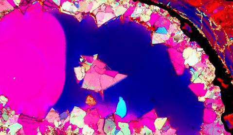
Figure 5.1:  A photomicrograph of Dolomite and Calcite Crystallites taken through an optical microscope.  The photograph is from the dinosaur bone collection [61].

 

            My approach will be to perform ab-initio calculations on small clusters (N = 1à 4) of CaCO₃ and then perform a fit of the parameters of the RIM potential to the results of the ab-initio calculation.  Once the parameters of the RIM potential are refined, I will use the simulated annealing method to determine the structures for larger clusters.   I will investigate the relationship between binding energy per molecule and the cluster size and investigate the rates of diffusion for the systems.  

 

5.2    Rigid Ion Model Potential

 

The interatomic potentials for CaCO₃ polymorphs have been modeled using the Rigid Ion Model (RIM), or two-body Born-Meyer type potential, supplemented by coulomb interactions between point charges and angular and torsional terms in the CO₃ group [18].  In the RIM potential the atoms are assumed to be point charges based on the electronic properties of the atom when participating in ionic bonds.  The RIM is a sum over the pair potentials between atomic pairs and is defined as follows:

 

 

            (5.1)

 

 

where

 

                                                                  (5.2)

                                                 (5.3)

                                                      (5.4)

                                                (5.5)

 

 

Here  ‘Z_i’ (i=Ca, C, O) are the point charges on the various atoms, A_ij, r_ij, and c_ij are the parameters.  The potential energy terms defined above are the different interactions that exist between atoms within the molecular structure.  The coulomb interaction between the ions of different charge signs is the major contributing factor to the stability of the crystal lattice in the bulk material.   The exponential term is always a positive quantity and represents the short-range repulsive force caused by the overlap between the outer-shell electrons of the atom.  This is the main factor that counteracts the attractive coulomb term and contributes to the stability of the lattice.   The 1/r⁶ term is a dispersive attractive force in the O-O interactions and results from the instantaneous dipole-induced dipole interaction.  Additionally, two equations governing the angular restoring forces associated with the CO₃ group are added to the RIM potential:

 

                                                (5.6)

 

 

where k_q, k_y are the restoring constants from the angular deviation from the equilibrium values,  q₀ and y = 0^o.  The first potential energy term, V_q, defines the restoring potential with respect to the bond angle O-C-O where the instantaneous bond angle is q.  At equilibrium the bond angle, q, is 120^o.  The second energy equation is the torsion term, V_y, which tends to keep the CO₃ group planar.  The equilibrium value for y is 0^o.

Originally the parameters were determined empirically by fitting the values to the bulk properties such as lattice constants, elastic moduli, and phonon data, obtained from lattice dynamics and experiments. The parameters reported in the literature by Pavese et al. [18] are reproduced in Table 5-1.

 

Table 5.1:  Table of parameters in the RIM Potential from Ref. [18].

 

 

 

In this study we will make a refinement to the parameters by fitting them to the results of ab-initio calculations of small CaCO₃ clusters. 

 

5.3    The Structure and Energetics of Calcite Obtained with DFT

 

I began the analysis of calcium carbonate structures by performing ab-initio calculations using B3PW91/6-311g(d) on clusters of CaCO₃ molecules.  This is the same method and basis set used in the analysis of calcium clusters.  To find a starting geometry for the runs, I used different cuts from the lattice by selecting random geometric arrangements of the CaCO₃ molecule, and performed a geometry optimization using the RIM Potential with Pavese’s parameters.  Once a number of geometric optimization were performed using the RIM potential, with the parameters defined by Pavese et al. [18], I used that geometry as input to the Gaussian98 package in performing a full optimization containing up to four molecules of CaCO₃.

The various isomers found are shown in Fig. 5.2, 5.3, and 5.4.   The single molecule, Fig. 5.2, reveals a geometry that is planar and has C_2v symmetry.  This is the only optimized geometry for the molecule.  When I optimized two molecules of CaCO₃, I obtained the two low energy structures shown in Fig. 5.2, having C_2h and C_2v symmetry.   The structure on the left, with C_2h symmetry, has the lowest energy, while the structure on the right, C_2V, has the next to the lowest energy.  For three molecules of CaCO₃, a “ring” structure was found as in Fig. 5.3.  The lowest energy structure has the C_S symmetry, while the structure having C_3V symmetry has the next to the lowest energy.  For clarity I show a side view of the geometry for each structure.  There are several minima for four molecules of CaCO₃, Fig. 5.4.  However only the two lowest energy structures are shown in the figure.  The left figure shows a top view of the structure while the right view shows the geometry from the side.  The top geometry is the lowest energy structure, having C₃ symmetry and the bottom structure has C_S symmetry.  Structures containing more than four molecules were too computationally demanding for ab-initio calculations.  In all the structures we found that the lower energy structures were the ones that had kept the CO₃ group as a planar triangle.

 

 

 

Figure 5.2:  The lowest energy structure of CaCO₃ and the two lowest energy structures for (CaCO₃)₂, optimized using the GGA.  The lowest energy structure for (CaCO₃)₂ is the left structure.

 

The binding energy of a cluster of molecules was found by taking the difference between the optimized energy of the structure and the sum of the energy of the atoms within the cluster.  The summation of the energy of the individual atoms, calcium, carbon, and oxygen, for one molecule of CaCO₃ gives a value of –940.1113353 au (one calcium atom, one carbon atom, and three oxygen atoms).  Table 5.2 shows the calculated energy of each atom within a CaCO₃ molecule and the optimized energy and C-O distance in the CO₃ radical.  Tables 5.3 and 5.4 show the symmetry, total energy, binding energy, average bond lengths, average charges on the atoms, dipole moment, and characteristic frequencies of vibration of the cluster structures depicted in Fig. 5.2, 5.3, and 5.4. 

 

 

 

 

 

 

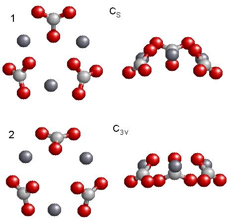
Figure 5.3:  Top (left) and side (right) views of the two lowest energy structures for three molecules of CaCO₃ that were optimized using GGA methods.  The lowest energy structure is the C_s structure.  The side views (on the right) are given to aid the visualization in 3D.

 

 

 

 

 

 

 

 

Figure 5.4:  Top (left) and side (right) views of the two lowest energy isomers of (CaCO₃)₄.  The lowest energy structure is the C₃ structure.

 

 

Table 5.2:  Atomic energy using B3PW91/6-311g(d).

 

 

 

 

Table 5.3:  CaCO3 clusters.  Symmetry, energy, and binding energy using B3PW91/6-311g(d) correspond to structures in Figs. 5.2-5.4.

 

 

Table 5.4: The average bond length, average charge on the atoms, Dipole moment, and vibrational frequencies of the (CaCO3)_n structures of Table 5.3.

 

 

 

The experimental value for the C-O bond length in bulk matter is 1.281 Å [59], which is in close agreement to our average value of 1.30 Angstroms.

The binding energy per molecule as a function of cluster size is shown in Fig. 5.5 for the lowest energy structures. The geometric optimization using the GGA method (blue) was on structures containing up to four molecules of CaCO₃, while structures optimized using the RIM potential (red) with published parameters of Table 5.1, was used on structures containing up to ten molecules.   Due to the computationally intensive calculations required in the GGA method, we were only able to perform calculation for up to four molecules of CaCO₃.  There is a large increase in binding energy per molecule in going from one to four molecules of CaCO₃.  The curve abruptly changes with two molecules, where there is a much slower and gradual increase in binding energy per molecule with each additional molecule.  Although we have only four data points for the GGA method we can still make some comparative studies.  The RIM potential, using the parameters from Pavese et al. [18], overestimates the binding energy for all cluster sizes except one molecule.  For one molecule of CaCO₃ the RIM potential underestimates the binding energy.  Both the ab-initio calculations and the RIM potential have the same general behavior for clusters containing more than two molecules.  The structure obtained with the RIM potential is the same obtained in the lowest energy isomer with GGA up to four molecules.

The ionization potential (IP) and electron affinity (EA), Table 5.5, were calculated for each of the lowest energy structures, for N = 1 à 4.  The IP increased from 8.3 eV to 8.7 eV in going from one to two molecules, but for three and four molecules the IP did not change significantly.  The EA also increased from –1.39 eV to –0.54 eV in going from one to two molecules, however there was no significant change for three and four molecules.  This calculation was done in the frozen geometry approximation.  It is interesting to note that in these molecular clusters the IP doesn’t decrease with increasing number of atoms as it does in metallic clusters.

 

 

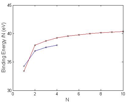
Figure 5.5:  Plot of the binding energy per CaCO₃ molecule vs. number of molecules for the lowest energy structures using the B3PW91/6-311g(d) method (blue) and the RIM potential (red).  The structures of the RIM potential were optimized using the parameters given by Pavese et al. [18].

 

 

 

Table 5.5:  Table of ionization potential and electron affinity for the lowest energy structure for (CaCO₃)_n, with n=1à4.

 

N	Ionization Potential (eV)	Electron Affinity (eV)
1	8.30	-1.39
2	8.70	-0.54
3	8.92	-0.35
4	8.83	-0.53

 

 

5.4    Improved RIM Potential Parameters

 

From Fig. 5.5, I can say that there are significant differences between the binding energy from the ab-initio calculation and the binding energy of the optimized structures using the original parameters of the RIM potential.  There is not much of a deviation between the geometry of the structures.  A computer program was written that would fit the parameters of the RIM potential to the results of the ab-initio calculation using a “crude” method in combination with Newton’s method to minimize the mean square error.  The fitting was done on the binding energy and the geometric structure as described in Chapter 2.  In the fitting of the parameters I began with an initial guess using the parameters of Pavese et al. [18].  Table 5.6 lists the parameters.  Some of the parameters had insignificant changes; therefore they were not included in the fitting.   From Table 5.7 we can see an improvement between the binding energies for two, three, and four molecules, although there was only a slight improvement in the geometry of the structures.  The standard deviation reported in Table 5.7 corresponds to Eq. 2.21 for the bond distances. 

 

Table 5.6:  A list of the new RIM parameters and those defined by Pavese et al. [18]. 

 

 

Parameter	Old Parameters [18]	New Parameters
ACa-O	1870.29 eV	1770.46 eV
AC-O	54129.49 x 108 eV	54129.49 x 108 eV
AO-O	14683.52 eV	20427.85 eV
rCa-O	0.2893 Å	0.2930 Å
rC-O	0.0402 Å	0.0402 Å
rO-O	0.2107 Å	0.207477 Å
ZCa	2.0 e	1.9927 e
ZO	-0.995 e	-0.9801 e
ZC	0.985 e	0.9477 e
cij	3.47 eV x Å6	2.914 eV x Å6
kq	2.55eV	2.55 eV
kf	0.0917 eV	0.0197 eV
q (O-C-O)	120.0	120.0
sE	3.77 eV	1.57 eV

 

 

Table 5.7:  A comparison between the energy and the geometry using the parameters given by Pavese et al. [18] and the new parameters.  

 

 

 

5.5    The Annealing Method Applied to CaCO₃ Clusters

 

The next step in my analysis was to use the new parameters in the RIM potential to find the structures for larger clusters of CaCO₃.  For structures of calcium carbonate containing more than ten molecules, Fletcher-Reeves-Polak-Ribierre minimization method described in Numerical Recipes [64] was inefficient for the optimization of structures; therefore, we used the simulated annealing method in locating minimum energy structures.  The simulated annealing method is based on the annealing of materials in a laboratory, where the physical process of heating and then slowly cooling a substance will avoid the trapping of the system in metastable states.  The hope is to achieve structurally strong energy configurations with the lowest possible energy.  The repetitive heating and cooling of the material will result in a more compact structure.  For a large system of atoms this can be a very efficient method to find the low minimum energy structure.  The heating and slow cooling gives an opportunity for the structure to jump out of local minima with a reasonable probability and search for a lower energy structure.  The simulated annealing method is an optimization approach for minimizing atomic or molecular systems once a potential function is given.  To apply simulated annealing, the molecular system is initialized from a given set of atomic coordinates and random velocities.  At each time step the atoms are moved in accordance to the net forces acting on the atom as resulting from the RIM potential.   The equations of motion of each atomic coordinates are solved using velocity-verlet method.  At time step ‘i’, the position of the atom is moved to a new position as in equation 5.7.  The velocity is also calculated by knowing the forces at time step ‘i’ and ‘i-1’, as in equation 5.8.

 

 

                                         (5.7)

 

 

                                               (5.8)

 

where ‘r’ and ‘v’ are the positions and velocity of each atom in the system, ‘F’ is the force acting on each atom at time step ‘i-1’ and ‘m’ is the mass of the atom.  The time step, Dt, is very small.  The atomic force is calculated from the RIM potential at each new geometry:

 

                                                         (5.9)

 

where ‘V’ is given in Eq. 5.1.  The cycle is repeated for the next time step.

In applying this to the simulated annealing method, I began with a cut from the lattice and ran it through 10,000 time steps to equilibrate the cluster.  The temperature of the system during the equilibration was approximately 800-900 K.  The time step was chosen to be 1.0 x 10^-15 seconds.  At the end of the equilibration the velocity and atomic coordinates of each atom were saved to a file.  The file was then used as input to the simulated annealing algorithm.   During the simulated annealing process the atoms are heated up by increasing the velocity of each atom, followed by a cooling, or a decrease in the average kinetic energy.   The cycle is repeated for 10,000 time steps, at which time the system is allowed to quench to a minimum energy state by setting the velocity to zero.  By the repetitive heating and cooling of the clusters, the molecular system can jump out of a local minimum energy configuration in to another of lower energy.  For the larger clusters I observed that occasionally the C-O bond in the CO₃ group would break resulting in a free oxygen atom.  These simulations were discarded.  This was avoided in the minimum energy structure by using different velocity and geometries until there was no breaking of the C-O bond.

 

 

 

Figure 5.6:  Plot of the binding energy per CaCO₃ molecule vs. number of molecules for the lowest energy structures using the RIM potential with the new parameters and the annealing algorithm.  The ab-initio points (red circles) are plotted for comparison.  The RIM potential with old parameters is given for comparison (triangles).

 

 

A plot of the binding energy per molecule vs. number of molecules, as in Fig. 5.6, resulted in a rapid increase in binding energy per molecule for small cluster sizes up to ten molecules followed by a leveling off of the binding energy/ molecule at approximately 39.2 eV/molecule.  A second plot of the binding energy per molecule vs. the reciprocal of the number of molecules, as in Fig. 5.7, has an approximate linear relationship.  The y-intercept, corresponding to an extrapolated infinite cluster size results in a binding energy per molecule of approximately 39.4 eV per molecule.   In the small cluster size regime, when I did calculations for subsequent values of N (number of molecules in the molecular cluster), a stability pattern can be discovered by plotting the second difference of the binding energies at zero temperature.  This is shown in Fig. 5.8 where peaks indicate more stable clusters vis-a-vis of their neighboring sizes.  The cluster with seven molecules seems to be relatively more stable.

 

 

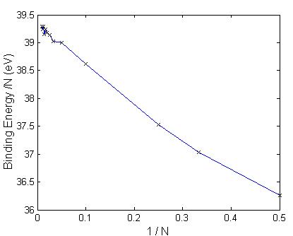
Figure 5.7: Plot of the binding energy per CaCO₃ molecule obtained with RIM and new parameters vs. 1/N, where N is the number of molecules.

 

 

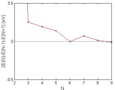
Figure 5.8:  Energy stability of the calcium carbonate clusters using the RIM potential at zero temperature for cluster sizes of two to nine molecules.

 

5.6    Diffusion Mechanism in CaCO₃ Clusters

 

When a system of atoms that is in a minimum energy state is heated, the atoms within the cluster will jump between local potential energy wells.  The atoms will move within a cluster depending on the potential energy surface.   I begin by defining the mean square displacement at time ‘t’ as

 

 

                 (5.10)

 

where u² is the instantaneous value of the mean square displacement per atom from their initial coordinates, x₀, y₀, z₀, N is the number of atoms, and x_i(t) y_i(t) z_i(t) are the final atomic positions at 10,000 time steps.  The mean square displacement is a measurement of how much the atoms move from their original to their final positions.  The average kinetic energy of the system is adjusted until the temperature, which is usually time averaged over 10 time steps, has the desired value.  Once the desired temperature is reached, the atoms and molecules are allowed to move freely within the system in a manner dependent on the local potential energy for a period of 10,000 time steps.  This is repeated for a number of different temperatures.  The temperature is defined in terms of the average kinetic energy:

 

                                           (5.11)

 

where k is Boltzmann’s constant and the brackets refer to a time average.  Since coordinates and velocities are referred to the center of mass, these degrees of freedom do not enter in the calculation.  Initial conditions were also adjusted to have zero angular momentum.  In scaling the temperature I use the ratio

 

                                              (5.12)

 

where ‘act’ and ‘des’ refer to the actual and desired temperature and kinetic energy.

In a monoatomic system, the relationship between the self-diffusion coefficient and the mean square displacement is

 

                                                       (5.13)

 

where the time, t, is a very large time interval.  The equation for the self-diffusion coefficient as a function of temperature is assumed to follow an Arrhenius temperature dependence given by

                                                          (5.14)

 

where e is the activation energy, k is Boltzmann’s constant, and T is the average temperature for the 10,000 time steps.  The activation energy is the effective energy barrier that exists between local minima of the energy surface.  For a molecular cluster, there are several points to remember.  First, the system is not monoatomic, therefore Eq. 5.14 is only an approximation if Eq. 5.10 is used for the mean square displacement.  Second, in a cluster there is an overall rotation of the cluster at finite temperatures that could mask considerably the mean square displacement.  Thirdly, since the cluster has a finite volume, the linear dependence of u²(t) and ‘t’ will not be achieved at very long times.  Instead one would expect that u²(t) would reach a maximum value at t à infinity, consistent with the volume of the cluster.  The first two points can be redefined by choosing a weighted average where each displacement ‘i’ is weighted by m_i/M, where m_i is the mass of each atom and M is the total mass of the cluster.

 

                                        (5.15)

 

 In the case of the cluster rotation, it is possible to set initial conditions on both positions and velocities such that the total angular momentum of the cluster is zero.  Unfortunately it is not possible to avoid the third point.  Therefore, in clusters and idea of the value of ‘D’ can only be obtained at relatively short times, where the mean square displacement still behaves linearly with time.

In the Molecular Dynamics simulation carried out here, the total simulation time is 10,000 time steps, or 10^-11 seconds.  In this simulation, I will investigate the relationship between the self-diffusion coefficient and temperature and determine the activation energy.   Besides this, five different initial conditions were chosen, and runs of 10,000 time steps initialized from each of them.  Then Eq. 5.15 was averaged over these five runs.

            When performing the simulation to calculate the self-diffusion coefficient it is important that three conditions be satisfied; the center of mass is at the origin, the total linear momentum of the system is zero, and the total angular momentum of the system is zero, i.e. no rotation.  For the linear and angular momentum to be zero, I have chosen that the initial velocity of each atom in the cluster be assigned a value of zero.  This certainly ensures that the linear and angular momentum of the molecular system will be zero throughout the simulation since there are no external forces driving the system.  A correction is made to the position vector, ‘r’ of each atom in the cluster so that all the atomic coordinates will be relative to the center of mass of the cluster.

      

                                           (5.16)

                                               

where ‘r’ is the atomic coordinates, ‘m’ is the mass of the atom, and ‘M’ is the sum of all the masses in the cluster.  The position of the center of mass, linear momentum, and total angular momentum was observed to be nearly zero throughout the simulation.   It is important that the cluster does not move or rotate during the simulation or the results would be in error.  The cluster, which is already at a minimum energy, is given energy by displacing the positions of the atoms in the cluster by a small distance to give the system enough potential energy to start the system in motion.  The temperature of the system is increased to the desired amount by using Eq. 5.12 for 20 time steps.  The system is allowed to equilibrate for an additional 10,000 time steps.  From 10,000 to 20,000 time steps in intervals of 10 time steps, the time, temperature, and the square displacement of each atom is recorded.

            Tables 5.8 and 5.9 contain the temperature, mean square displacement of each type of atom (Ca, C, O), and the self-diffusion coefficient for 150-atom and 250-atom clusters.  In the diffusion process the atoms move between local minima on the potential energy surface, if there is enough energy present to overcome the local energy barriers.  For small temperatures there is insufficient energy to overcome the barrier and the atoms remain confined to the proximity of the initial minimum.  As seen in Fig. 5.9 and 5.10 there is no appreciable movement of the atoms within the cluster at about 300 K since the mean square displacement is hardly increasing with time.  It is only when there is enough kinetic energy that the atoms begin to move between regions of different minima.  It took a temperature of about 1180 K for any appreciable atomic diffusion within the 150-atom cluster.  For the 250-atom cluster the temperature required for any appreciable diffusion was about 1205 K.  This seems to indicate that there is smaller mobility within the larger clusters than in the smaller clusters.  By finding the slope of the lines on the log plots in Fig. 5.11, I can determine an estimate of the activation energy.  In calculating this estimate I ignored the data point that corresponded to the lowest temperature of 308 K.  The error bars in the figure correspond to twice the standard deviation of the temperature.  For the 30-molecular cluster, the plot in Fig. 5.11a is not linear and it is difficult to extrapolate a value for the activation energy.  For the 50-molecular cluster, Fig. 5.11b seems more linear, in which case an estimate of about 0.1 eV can be given to the activation energy.  That value is consistent with the previous observations that there is diffusive behavior only at temperatures above 1000 K. 

 

 

Table 5.8:  Average values over five initial conditions of a 30-molecule cluster of temperature, mean square displacement, and self-diffusion coefficient at t = 10,000 time steps.  The uncertainties are twice the standard deviation.

 

 

 

 

Table 5.9:  Average values over five initial conditions of the 50-molecule cluster of temperature, mean square displacement, and self-diffusion coefficient at t = 10,000 time steps.  The uncertainties are twice the standard deviation.

 

 

 

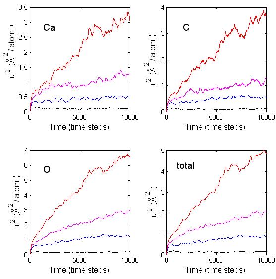
Figure 5.9:  Mean square displacement per atom for calcium, carbon, oxygen, and the sum of the displacements at temperatures 308 K (black), 690 K (blue), 964 K (magenta), and 1179 (red) for a 30-molecules cluster at several temperatures.

 

 

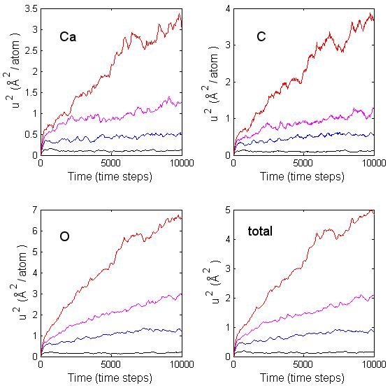
Figure 5.10:  Mean square displacement per atom for calcium, carbon, oxygen, and the sum of the displacements at temperatures 308 K (black), 684 K (blue), 964 K (magenta), and 1205 (red) for a 50-molecules cluster.

 

 

 

 

 

 

Figure 5.11:  Logarithm of the diffusion coefficient D/D₀ vs. the reciprocal of the average kinetic energy, (a) 30-molecular cluster with D₀ = e¹⁰ Å /s.  (b) 50-molecular cluster with D₀ = e¹⁰ Å /s.    

 

5.9    Conclusion

 

In the research on clusters of CaCO₃, ab-initio calculations were performed for structures containing one to four molecules.   Global minimum energy structures were found for the structures and the binding energy per molecule vs. number of molecules was plotted for up to 4 molecules.  Optimized structures were also found using the RIM potential with the parameters from Pavese for up to 10 molecules.  A plot of the binding energy vs. cluster size indicates that the Pavese-RIM potential overestimated the results of the ab-initio calculation in the range of cluster sizes one to four.  The plot of the RIM potential for clusters larger then 4 indicated a leveling off of the binding energy.  For one molecule of CaCO₃ the RIM potential underestimates the binding energy.  Both the ab-initio calculations and the RIM potential have the same general behavior for clusters containing more than two molecules.

The results of the ab-initio energy calculations and the optimized structures were used in the fitting of the parameters of the RIM potential.  An improvement in binding energy was observed between the RIM potential and the quantum mechanical results for two, three, and four molecules.  The parameters were used in a computer simulation using the simulated annealing algorithm and molecular dynamics to obtain the geometry and binding energies for structures containing up to 500 atoms, or 100 molecules of CaCO₃. A plot of the binding energy vs. 1/N reveals a close to linear relationship.  The intercept of the y-axis indicates that for clusters of infinite size the binding energy per N is 39.4 eV/molecule.   This can be compared with the cohesive energy of calcite that is 29.14 eV [68].

The mobility of atoms within the cluster was small for the cluster sizes and temperature range investigated.  The average displacement after 10,000 time steps was found to be of the order of some of the nearest neighbor atomic distances.   However, we did find an estimate of the activation energy for the clusters, which is 0.1 eV for the 50-molecule cluster.   This energy is of the order of energy differences between the different isomers of a small cluster.  In the three data points collected for the two clusters, the natural log of D/D₀ versus the reciprocal of the average kinetic energy was about linear for the 50-molecule cluster but deviated from linear for the 30-molecule cluster.  A better determination of the activation energy can be done in the canonical ensemble.  For that to be possible I would need to carry out a complete set of different simulations using mainly Monte Carlo methods.  This is work that should be pursued in the future.